Navigate this guide · 2,019 words
The essential signal
- Attention is a learned weighted sum. Queries ask, keys label and values supply the content that gets blended into each position.
- The whole core fits in one line. Score queries against keys, scale by the square root of the key dimension, softmax into weights and sum the values.
- Multi-head attention and position codes turn that core into a full architecture. Heads capture different relationships while position signals restore word order.
- The cost grows with the square of sequence length. FlashAttention tiles the same exact computation and grouped-query attention shrinks the key-value cache.
The bottleneck before attention
Before 2017 the best language models read like careful students working through a sentence one word at a time. Recurrent networks carried a hidden state from word to word and updated it at each step. That design had a clear weakness. Everything the model had learned about the start of a sentence had to survive inside one state vector by the time the end arrived. Long sentences leaked meaning along the way. Training was slow for a second reason. Step ten could not run until step nine had finished so the work could not spread easily across many processors at once. [1][2][1]
Convolutional models eased the problem without removing it. They looked at local windows of words and stacked layers to widen the view. A distant relationship still needed many layers to bridge. Attention already existed as an add-on that let a decoder glance back at encoder states. The 2017 Transformer paper made a bolder claim. It built the whole architecture from attention alone and dropped recurrence and convolution entirely. The result trained faster and translated better. [1][3][1]
What attention actually computes
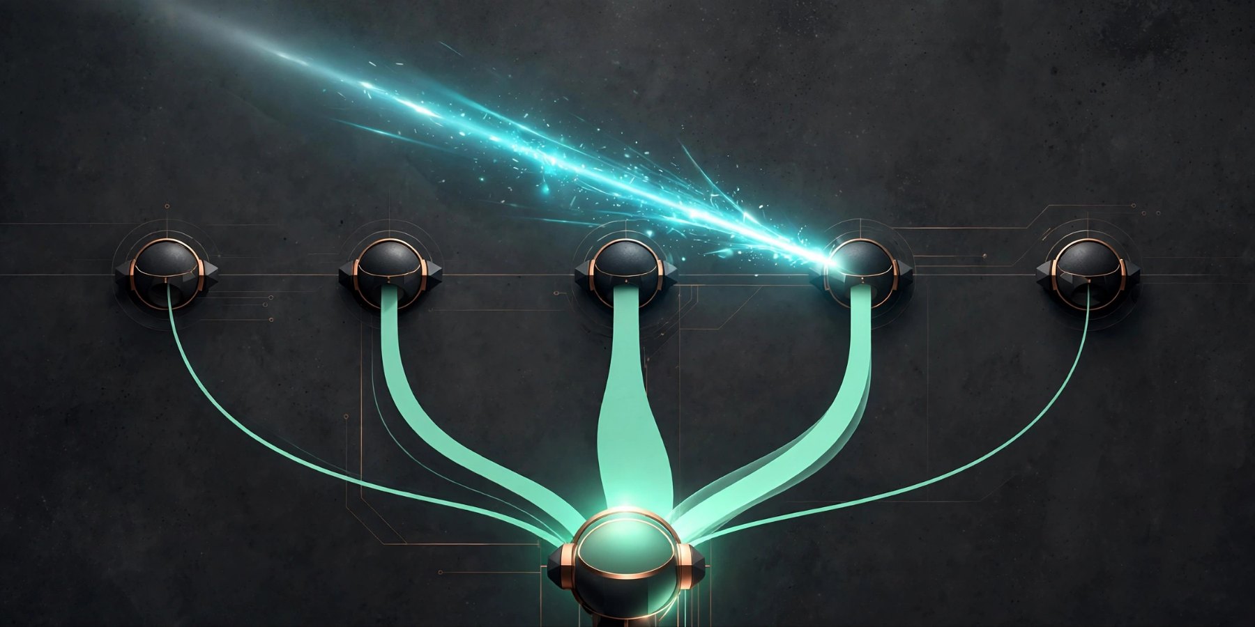
Strip away the diagrams and attention is a small idea. It maps one query and a set of key-value pairs to one output. The output is a weighted sum of the values. Each weight comes from a compatibility score between the query and the matching key. A high score means that value matters more for this position. A low score fades it toward zero. Nothing in the operation stores a fact or understands a sentence on its own. It only decides how much of each available piece of information should flow into the current position. [1][3][1]
That framing matters because it explains both the power and the limits of the mechanism. Attention gives every position direct access to every other position in a single step. A word at the end of a long sentence can draw on a word at the start without passing through a chain of intermediate states. The price is that every position must be compared with every other position. The operation is simple and the bill for running it grows fast. [1][2][1]
Queries, keys and values in plain language
Every token in a sequence gets three new vectors before attention runs. The query vector says what this position is looking for. The key vector says what this position offers as a label. The value vector carries the content that will actually move forward if this position is chosen. All three come from the same starting embedding but each passes through its own learned projection matrix. Training shapes those matrices so the comparisons become useful. [1][2][1]
A useful way to picture it is a set of labelled folders. The query is the question written on a slip. Each key is a label on a folder. The score measures how well each label matches the question. The value is the paper inside the folder. Attention reads the folders in proportion to their match scores and blends their contents into one new vector for the querying position. In the original paper the embedding vectors had 512 dimensions while the query, key and value vectors had 64. Smaller comparison vectors kept the multi-head version of the operation affordable. [1][2][1]
The score, the scale and the softmax
The score itself is a dot product. Take the query vector for one position and dot it with the key vector of every position in the sequence. A large dot product means the two vectors point in a similar direction and the match is strong. A small or negative dot product means weak relevance. Dot products are cheap to compute in bulk which is one reason the whole operation maps so well onto matrix hardware. [1][3][1]
Two more steps turn raw scores into usable weights. First the scores are divided by the square root of the key dimension. In the original paper that divisor was 8 because the key dimension was 64. Without scaling, long vectors produce large dot products that push the next step into flat regions where learning slows to a crawl. Then a softmax turns the scaled scores into positive weights that sum to exactly 1. Each value vector is multiplied by its weight and the results are added together. That sum is the attention output for one position. [1][2][1]
One worked walk-through
Take the sentence "The programmer told the designer that she had won the award." A reader knows at once that "she" is ambiguous. Grammar alone does not settle whether the programmer or the designer won. A model encoding "she" faces the same problem. Self-attention lets the position of "she" compare itself with every other word in the sentence and pull in a blend of the programmer and designer representations weighted by what training taught it about similar sentences. [1][2][1]
Notice what the mechanism does not do here. It does not resolve the ambiguity by reasoning about the world. It blends evidence. If the training data leaned one way then the blend leans that way too. That is why attention outputs feel smart and still make confident mistakes. The weighted sum is only as good as the projections that produced the queries, keys and values and the data those projections learned from. When you read an attention diagram showing bright lines between words, remember that brightness is a weight in a sum, not a proof of understanding. [2][3][1]
Why many heads beat one
A single attention pass can be dominated by the strongest match. In the sentence above, the word itself usually wins the largest weight and subtler relationships get drowned out. Multi-head attention answers that by running the operation several times in parallel with different projection matrices. The original paper used eight heads. Each head projects the same input into its own smaller subspace and computes its own set of weights. [1][2][1][2][3]
The heads are then concatenated and passed through one more learned projection that merges them back to the full model width. One head might end up tracking nearby words while another tracks distant ones. That assignment is never programmed in advance. It emerges from training because different projections capture different patterns in the data. The paper's own background section is honest about a related trade-off. Averaging many positions into one vector reduces resolution and multi-head attention is the countermeasure that keeps distinct relationships visible. [1][3][1][2][3]

Order without recurrence
Attention looks at all positions at once which creates a puzzle. Without extra help the model cannot tell "the dog chased the cat" from "the cat chased the dog" because the same words appear in both. The paper solves this by adding a position signal to each embedding before the first layer. The original design used sine and cosine waves of different frequencies. Each position gets a unique pattern and each dimension of that pattern oscillates at its own rate. [1][3][1][2][3]
The position code has the same size as the embedding so the two can be added directly. The paper also notes that learned position codes performed almost identically in its tests. Sinusoidal codes had one extra attraction. Their wave structure lets the model in principle extend to sequences longer than any it saw in training because position differences follow a predictable pattern. Later designs changed the details but the principle stayed. Order is not built into attention itself so it must be supplied from outside. [1][2][1][2][3]
The encoder, the decoder and the mask
The full Transformer stacks six encoder layers and six decoder layers. Each encoder layer has a self-attention sub-layer followed by a feed-forward network applied separately at each position. Residual connections carry the input around each sub-layer and layer normalisation steadies the result. Every sub-layer output keeps the same 512-dimensional width so the stack fits together cleanly. [1][3][1][3]
The decoder adds a third sub-layer. It attends over the encoder output so each generated word can consult the whole input sentence. Its self-attention is masked so a position can only attend to earlier positions and never to words that have not been generated yet. Combined with outputs shifted by one position, the mask guarantees that a prediction for position i depends only on known outputs before i. That single rule is what makes training on full sentences possible while generation still proceeds one word at a time. [1][3][1][3]

The price of looking everywhere
The strength of attention is also its bill. Every token compares itself with every other token so the work grows with the square of the sequence length. The FlashAttention paper states the point plainly. Standard self-attention has time and memory complexity that are quadratic in sequence length. Double a 4,000-token context to 8,000 tokens and the pairwise work roughly quadruples. That is why long context windows are expensive even before any other part of the model is counted. [4][8][4][5][7][8]
Generation adds a second cost. When a model produces text one token at a time it would waste enormous effort recomputing keys and values for every earlier token at each step. Systems therefore cache those keys and values and reuse them. The cache grows with sequence length and with the number of key-value heads. A model with many heads and a long conversation carries a large cache and serving it fast becomes a memory-bandwidth problem as much as a compute problem. [5][7][4][5][7][8]
How engineers made attention cheaper
FlashAttention attacked the memory side without changing the maths. It tiles the computation into blocks that fit in fast on-chip memory instead of writing the full score matrix to slower memory and reading it back. The output is exactly the same as standard attention. The paper reported a 15 percent end-to-end training speedup on a large BERT model and a 3x speedup on a GPT-2 scale model along with far lower memory use on long sequences. [4][7][4][5][6][7]
Grouped-query attention attacked the cache side. Standard multi-head attention keeps a separate key and value head for every query head. Multi-query attention shares a single key and value head across all query heads which speeds up decoding but can cost quality. Grouped-query attention sits between the two. Query heads are split into groups and each group shares one key and value head. The paper showed that uptrained grouped-query models reached quality close to multi-head attention with speed close to multi-query attention. [5][6][4][5][6][7]
What attention does not do
Three misunderstandings show up again and again. First, attention weights are not explanations. A bright weight says a value contributed heavily to a sum. It does not say why in human terms and a model can reach the same output through many different weight patterns. Second, attention does not remember facts between prompts. The weights of a trained model live in its projection matrices and feed-forward layers. Attention itself only routes information within the current sequence. Third, longer context does not guarantee sharper focus. As more tokens compete for weight, each individual weight shrinks and the signal from any one passage can wash out. [1][3][1][2][3]
None of this diminishes the idea. It clarifies where the idea ends and the rest of the system begins. Embeddings carry learned meaning, feed-forward layers transform it, training shapes every projection and decoding rules decide how outputs are chosen. Attention is the routing layer that lets those parts talk across distance in a single step. Judging a model by its attention maps alone is like judging a library by its catalogue cards. The catalogue matters enormously and it is not the books. [2][3][1][2][3]
How to read the paper yourself
Start with the abstract and the background section of "Attention Is All You Need" before touching any equation. The abstract states the bet in a few lines. The model drops recurrence and convolution entirely and still beats the best translation results of its time, which is why the field paid attention. [1][2][1][2][3]
Then read the model section with a notebook open beside it. The Harvard annotated version walks through the same architecture line by line with working code and Jay Alammar's illustrated guide builds the intuition picture by picture. Try three small experiments once the basics click. Mask a decoder by hand and watch a future word disappear from the allowed set. Change the number of heads in a tiny implementation and watch the subspaces change. Feed the ambiguous sentence from earlier in this article through a small model and inspect which words the "she" position leans on. You will learn more from those three exercises than from rereading the maths twice. [2][3][1][2][3]
Questions, answered.
What is the difference between attention and self-attention?
Attention is the general operation. Self-attention is the special case where the query, key and value sequences all come from the same input. Encoder layers use self-attention so each word draws on other words in the same sentence. Decoder layers add cross-attention where queries come from the output being generated while keys and values come from the encoder.[1][3]
Why divide the scores by the square root of the key dimension?
Dot products grow with vector length. Large scores push the softmax into regions where its outputs barely change and gradients vanish, which stalls learning. Dividing by the square root of the key dimension keeps the scores in a range where the softmax stays responsive. In the original paper the key dimension was 64 so the divisor was 8.[1][2]
How many attention heads should a model have?
There is no universal number. The original paper used eight heads with a model width of 512 and a key dimension of 64 per head. More heads add subspaces but each head gets narrower. Modern models choose the count alongside model width, head size and cache budget. The right question is not how many heads but how much distinct information each head can carry at its size.[1][2]
Does a high attention weight mean the model understands that word?
No. A weight only records how much of one value flowed into one output position during one computation. It is a routing decision shaped by training, not a reasoned judgement. Two different weight patterns can produce similar outputs and a strong weight can reflect a statistical habit of the training data rather than a fact about the sentence.[1][3]
Why is long context so expensive?
Every new token must be compared with every token before it and the cache of keys and values grows with the sequence. The pairwise work scales with the square of length while the cache scales with length, head count and layer count. Tiled exact algorithms and shared key-value heads reduce the constants but the underlying growth stays.[4][5][7][8]
Where should a student start with this topic?
Read the original paper's abstract and model sections first, then work through an illustrated guide for intuition and an annotated implementation for code. Build a tiny attention layer yourself and test it on ambiguous sentences. The mechanism is small enough to implement in an afternoon and that afternoon will change how you read every later paper about large models.[1][2][3]
Read the sources.
- Attention Is All You NeedarXiv · Accessed 2026-11-08
- The Illustrated Transformerjalammar.github.io · Accessed 2026-11-08
- The Annotated TransformerHarvard NLP · Accessed 2026-11-08
- FlashAttention: Fast and Memory-Efficient Exact Attention with IO-AwarenessarXiv · Accessed 2026-11-08
- GQA: Training Generalized Multi-Query Transformer Models from Multi-Head CheckpointsarXiv · Accessed 2026-11-08
- Demystifying GQA - Grouped Query Attention for Efficient LLM Pre-trainingTowards Data Science · Accessed 2026-11-08
- Fastest LLM Inference: Lowest Latency and Most Tokens per Secondsafeguard.sh · Accessed 2026-11-08
- Human Brain vs LLM Context Window: Memory, Attention and AI Securitysafeguard.sh · Accessed 2026-11-08
Contributor articles and source links do not guarantee error-free reporting. See our editorial policy.